numpy.gradient() in Python: An Easy Guide

The numpy.gradient() function is a powerful tool for calculating the gradient of array inputs. The concept of the gradient is essential in fields like data analysis and scientific research, where it is used to create graphical representations of changes in large datasets. Let’s understand this concept before diving deep into the numpy.gradient function.

Understanding the Gradient

The gradient is a core idea in calculus and vector analysis. Essentially, it shows how fast a function changes or its slope in many dimensions.

For example, if you’re looking at a graph of temperatures over time, the gradient would show you not only which way the temperature is changing (getting hotter or colder) but also how fast it’s changing at each moment. This can be helpful for all sorts of things, like predicting the weather or understanding how things are changing in a scientific experiment. Essentially, it’s a tool that helps you understand how things are moving and changing in your data.

Let’s say we have a list showing temperatures recorded at different times(gap of 1 sec):

temperatures = [20, 22, 24, 21, 19, 18, 17]

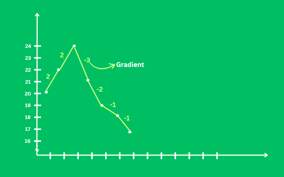
The gradient will show us the rate of temperature change over time:

[2.  2.  -3.  -2  -1.  -1.]

This is how we calculated it:

Between the first and second measurements, the temperature rises by 2 degrees.
Between the second and third measurements, it rises by 2 degrees.
Between the third and fourth measurements, it decreases by 3 degrees.
And so on.

Introducing numpy.gradient

Numpy offers us a function that can help us implement the concept we just learned. In NumPy, the numpy.gradient() calculates gradients for arrays. Gradients show how values in an array change in various directions.

Syntax:

Here is how we can use this function:

numpy.gradient(f, *varargs, axis=None, edge_order=1)

f: It is the Input array.
varargs: This is the spacing between values in f.
axis: It is the axis for computing the gradient. By default, it considers the last axis.
edge_order: The order of the edge for gradient computation. The default is 1.

Working:

This function calculates the gradient by using finite differences, which can be forward, backward, or central.
In a 1-D array, it finds the gradient at each point using first-order differences.
For arrays with more dimensions, it computes gradients along each dimension specified by the axis parameter.

Applications:

Image Processing: Gradients help in detecting edges in images using algorithms like Sobel and Prewitt.
Physics: Gradients are vital in simulations that involve fields such as temperature or velocity, as they determine how these quantities change in space.
Machine Learning: Gradients are essential in optimization algorithms like gradient descent, where they help update model parameters to minimize the loss function.

Considerations:

Spacing: If the spacing between values in the array is not uniform, you may need to specify it using the varargs parameter.
Edge Handling: The edge_order parameter determines how gradients are computed at the edges of the array. Lower values may result in artefacts, while higher values increase computational costs.

Examples of numpy.gradient in Python

Little confused? Don’t worry, let’s understand it better with some basic examples:

Example 1:

Let’s start with the basic array data.

import numpy as np

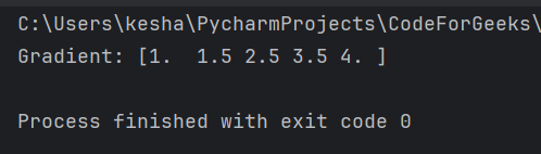
arr = np.array([1, 2, 4, 7, 11])

grad = np.gradient(arr)
print("Gradient:", grad)

In the output, each element of the gradient array represents the average rate of change between adjacent elements in the original array.

But according to our logic:

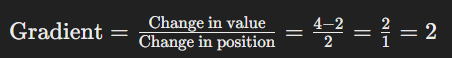
However, the output at the second position in the gradient array is 1.5. This is because the np.gradient() function computes the gradient using central differences, which takes into account the changes between adjacent elements on both sides. So, while the difference between 2 and 4 is indeed 2, the gradient considers the changes on both sides, leading to an average rate of change of 1.5.

Example 2:

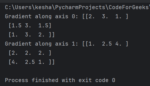
If we take a 2D array, we can specify the axis of calculation. Here’s how we do it:

import numpy as np

arr = np.array([[1, 2, 6],
                [3, 5, 7],
                [4, 8, 9]])

grad_axis_0 = np.gradient(arr, axis=0)
print("Gradient along axis 0:", grad_axis_0)

grad_axis_1 = np.gradient(arr, axis=1)
print("Gradient along axis 1:", grad_axis_1)

The np.gradient() function calculates the rate of change along rows when used with axis 0, creating a new array grad_axis_0. Similarly, when used with axis 1, it computes the rate of change along columns, resulting in a new array grad_axis_1.

Example 3:

Now, let’s see how we can apply edge orders.

import numpy as np

arr = np.array([1, 2, 4, 7, 11])

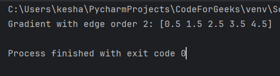
grad_edge_2 = np.gradient(arr, edge_order=2)
print("Gradient with edge order 2:", grad_edge_2)

The function finds the gradient with an edge order of 2. This means it calculates the gradient considering second-order differences at the edges of the array.

Conclusion

The numpy.gradient function is valuable for analyzing data in various aspects of daily life, such as stock market trends and weather changes. A huge amount of data is used for such computations and tools like this make it easy for us to graphically represent these large datasets.

Other NumPy functions for data analysis and manipulation are:

Don’t forget to explore these as well.