
New to Rust? Grab our free Rust for Beginners eBook Get it free →
Linear Regression Model for Data Points
Today we are going to learn about the linear regression model. We are going to learn about plotting or creating a linear regression model for all data points. In this article, we are going to learn or plot this model for a linear equation as well.
Before getting into it, we need to understand one more important which is regression analysis. it is a statistical algorithm to show the relation between two variables in a linear equation.
What is regression analysis?
Regression analysis is a form of predictive modeling technique that investigates the relationship between a dependent and independent variable in an equation. It involves graphical lines over a set of data points that most closely depict the overall set of data.
It shows the rate of change in the dependent variable on the y-axis by a short change in the independent variable on the x-axis.
Also read: Regression vs Classification in Machine Learning
Three major uses of Regression analysis
Let’s look at the major uses of regression analysis in general.
- Determining the strength of predictors: It measures the effect of the independent viable in the dependent variable.
- Forecasting the effect: Determining the effect of the independent variable on the dependent variable.
- Trend forecasting: It is used to get the point estimation by comparing and analyzing the errors between the expected values and data points.
Regression analysis is usually of two types as follows.
- Linear Regression: In this Regression, the prediction for continuous dependent value is obtained using the value of independent variables. The output/Prediction is the value of a continuous variable. The accuracy or goodness of the fit is measured by loss and the least square analysis algorithm.
- Logistic Regression: In this Regression, The probability of an event is obtained for predictive variables in a linear equation. It is used with the categorical variable. Here The output is between 0 and 1 as we are going to predict the probability or the normalized form of the occurrence of an event. It was been measured by accuracy precision like F1 score, ROC curve, confusion matrix, etc. The accuracy or goodness of the fit is measured by the Maximum likelihood estimation algorithm.
Today we will mainly focus on linear regression.
This regression is used to predict the continuous variables by classification and regression capabilities and to change the existing model by changing its threshold capacitance. Each value denotes the data points that could optimize the regression and it is not computationally expensive. The order of complexity usually falls on O(xn) and O(x2). The linear regression is easily comprehensible and transparent. those can be explained by simple mathematical notations and it is quite easy.
Linear regression use-cases
- If we take the case of business and marketing as well then we can get many uses as follows.
- evaluating trends and sales estimation.
- Analyzing the impact of price changes.
- Assessment of risk in financial services and insurance domain.
The linear regression analysis is been concluded by taking a linear equation y = mx + c. Where m is the slope and it shows the rate of regression that is positive or negative.When the value of the independent variable increases in the x-axis and the value of the dependent value increases in the y-axis then the regression is positive as well and when the value of the independent value increases in the x-axis but the value of the dependent value in the y axis decreases then the regression value is negative.
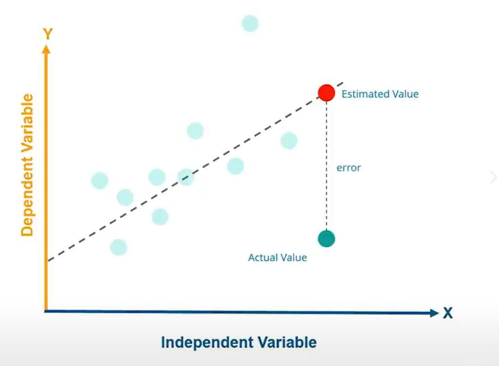
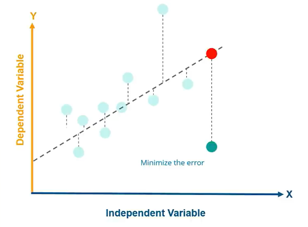
After plotting the Regression line to get an estimated value, We need to get the difference between the estimated value and the data points, that difference is the error. After getting the errors for each data point we need to get the minimum error by the least square method.
Let us move into our code snippet and do the same in terms of python code.
Step 1. Importing required modules
import pandas as pd
import numpy as np
import matplotlib.pyplot as plt
from sklearn.metrics import mean_squared_error
from sklearn.linear_model import LinearRegression
plt.rcParams['figure.figsize'] = (20.0, 10.0)
Step 2. Reading our Dataset
Let us read a dataset using pandas.read_csv() method and load the same to the variable named data. Here we are taking a dataset of babies containing two predictive variables head_size(cm^3) and weight(gram).
data = pd.read_csv('/content/dataset.csv', delimiter = ",", header = "infer")
print(data.shape)
data.head()
| index | Unnamed: 0 | Gender | age | head_size(cm^3) | weight(gram) |
|---|---|---|---|---|---|
| 0 | 0 | m | 1 | 4512 | 1530 |
| 1 | 1 | m | 1 | 3783 | 1297 |
| 2 | 2 | m | 1 | 4261 | 1335 |
| 3 | 3 | f | 1 | 3777 | 1282 |
| 4 | 4 | m | 1 | 4177 | 1590 |
Step 3. Fetch data from our dataset and load it into respective variables
#loading the head_size data into X variable as an array
X = data['head_size(cm^3)'].values

#Similarly loading the weight data into Y array
Y = data['weight(gram)'].values

#getting Mean for X and Y data points and loading the same into mean_x and mean_y respectively.
mean_x = np.mean(X)
mean_y = np.mean(Y)

#total no. of values
n = len(X)
Step 4: Plotting our Regression Graph
#creating our normalized equation for regression line by taking b0 as constant term and b1 as the slope
numerator = 0
denominator = 0
for i in range(n):
numerator += (X[i] - mean_x) * (Y[i] - mean_y)
denominator +=(X[i] - mean_x) ** 2
b1 = numerator/denominator
b0 = mean_y - (b1 * mean_x)
max_x = np.max(X) + 100
min_x = np.min(X) - 100
x = np.linspace(min_x, max_x, 1000)
y = b0 + b1*x
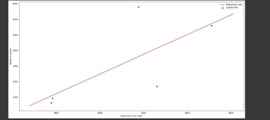
#plotting our regression line using normalized linear euation created ceated above
plt.plot(x, y, color='red', label = 'Regression Line')
#plotting out data points from the dataset
plt.scatter(X, Y, color='green', label = 'Scatter Plot')
plt.xlabel('Head size in cm cube')
plt.ylabel('Weight in grams')
plt.legend()
plt.show()
In the above code snippet, we just form our equation for the regression line (i.e. y = b0 + b1*x where b0 is a constant term and b1 is the slope ) and plotting our data points in the dataset taken.
Step 5: Getting our Prediction values
In this step, we will create our model using the LinearRegression() method and use the model to get the predictive value as well which is our main goal. along with the predictive value, we will get the mean error in our regression graph. Let’s follow the below code snippet for the same.
ss_t = 0
ss_r = 0
for i in range(n):
  y_pred = b0 + b1 * X[i]
  ss_t += (Y[i] - mean_y) ** 2
  ss_r += (Y[i] - y_pred) ** 2
r2 = 1 - (ss_r/ss_t)
X = X.reshape((n, 1))

#creting our model
reg = LinearRegression()
reg = reg.fit(X, Y)

#getting the predicted value for the dependent variable Y
Y_pred = reg.predict(X)

#getting the mean_squared_error as descibed in our diagrm above
mse = mean_squared_error(Y, Y_pred)

#calculating the final prediction by using the model and passing the data points as parameters and printing the same
r2_score = reg.score(X, Y)
print(r2_score)

#print the mean error getting the square root of mean_squared_error
print(np.sqrt(mse))
#We got the output as follows
       0.49777526481038026
       90.49284561870854
Conclusion
Today we discussed a very interesting topic which is Linear regression. We learned a little knowledge about Regression analysis as well. Hope you just go through our code snippet and got the same. We must visit again with some more exciting topics.