
New to Rust? Grab our free Rust for Beginners eBook Get it free →
Confusion Matrix – Understanding with examples
One of the most prevalent and in-demand technologies today is machine learning. It is equally crucial to evaluate the model’s performance as it is to design various models. The confusion matrix is employed to evaluate this performance and estimate other characteristics like the model’s accuracy and precision. It is mostly used for supervised learning models where the actual values are also provided. Other than this it is also helpful in cases of classification models.
In this article, we’ll attempt to clarify everything that you need to know about the confusion matrix, including what it is, why it is used, how it works, and how to implement it in Python programming language using various open-sourced packages.
Check: Python if…else Conditional Statement (With Examples)
What is Confusion Matrix
A confusion matrix is a matrix or layout used to evaluate how well a machine learning classification model functions. A confusion matrix helps us identify the correct predictions of a model for different individual classes as well as the errors. It does this by representing a table layout of the various outcomes of prediction and actual results of a classification problem. It is also helpful to evaluate factors like accuracy, recall, precision, etc.
Binary Classification Confusion Matrix
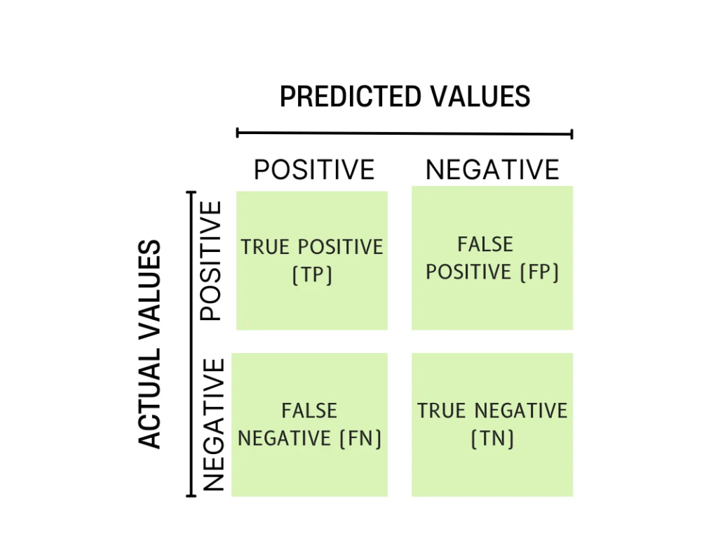
This is the simplest confusion matrix – a 2 X 2 table, with four quadrants below the confusion matrix. It is known as Binary Classification as it has two categories – positive (True) and negative (False). As you can see, we have our simple chart with predicted and actual results. In this case, the only predictions made are true or false or we can say Positive or Negative, hence this type of classification is called Binary Classification.
Understanding TP, FP, FN, and TN
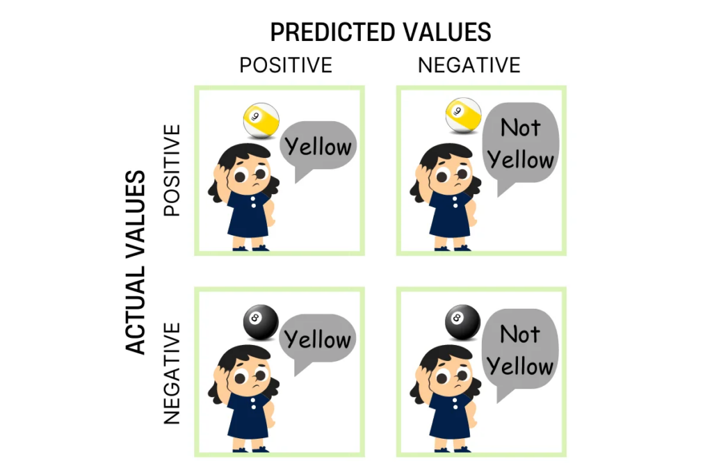
Let us try to understand these terminologies using an example. Suppose you have a ball and you ask your friend to guess the color of the ball. Now you know the actual color of the ball, your friend doesn’t know so she/he will predict the color of the ball. For simplicity let’s keep two predictions “Yellow” or “Not Yellow”. The overall result of this activity can lead to any of the following possibilities.
- True Positive (TP): If the ball is actually yellow in color and your friend predicts the “Yellow”. That means the actual value matches the predicted value, and the predicted value has no negation.
- False Positive (FP): If the ball is actually yellow but your friend fails to predict it correctly. That means the actual value doesn’t match the predicted value, and the predicted value has a negation. This is also known as a Type-1 error.
- False Negative(FN): If the ball is not yellow in color but your friend predicts it to be yellow. That means the actual value doesn’t match the predicted value, and the predicted value has no negation. This is also known as a Type-2 error.
- True Negative (TN): If the ball is not yellow and your friend predicts it correctly “not yellow”. That means the actual value matches with the predicted value and the predicted value has negation added to it.
Calculating Accuracy, Precision, and Recall
ACCURACY: The model’s accuracy indicates how frequently it was overall accurate. It is the proportion of all the examples that were successfully predicted in comparison to the total examples. Below is the formula for calculating the accuracy.
Accuracy = TP + TN / TP + TN + FP + FN
PRECISION: Positive predictions’ accuracy is determined using precision. It is the ratio of the true positive values of the example to all the predicted positives value – this means the summation of True Positives and False Positives. Following the formula for calculating the Precision.
Precision = TP / TP + FP
RECALL: It is also known as Probability of Detection or Sensitivity. It is the ratio of correct positive predictions to all the positive values – this means the summation of True Positives and False Negatives. Refer to the below formula for calculating the Recall in Confusion Matrix.
Recall = TP / TP + FN
The two terms Precision and Recall might seem confusing. To understand the difference between precision and recall, please visit here.
Also check: Top 25 Best Arduino Projects To Try in 2022
Implementing Confusion Matrix for Binary Classification
Before implementing the confusion matrix, we need to install and import a few packages that help to build the confusion matrix. Following is the code to import the required packages.
import numpy as np                                            # To provide actual and predicted values
from sklearn.metrics import confusion_matrix    # To build the confusion matrix
import matplotlib.pyplot as plot                         # To visualize the matrix
After importing we create two arrays one of the actual values and the other of predicted values. We pass these as parameters while creating the confusion matrix.
actual_values = np.array(['Yellow', 'Not Yellow', 'Yellow','Yellow','Not Yellow','Yellow','Yellow'])
predicted_values = np.array(['Not Yellow','Not Yellow','Yellow','Yellow','Not Yellow','Yellow','Yellow'])
confusion_mat = metrics.confusion_matrix(actual_values, predicted_values)
CM_view = metrics.ConfusionMatrixDisplay(confusion_matrix = confusion_mat, display_labels = ["Yellow", "Not Yellow"])
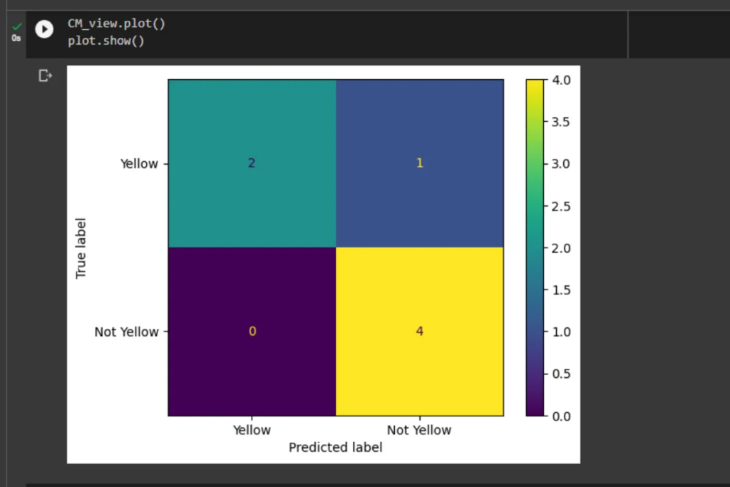
CM_view.plot()
plot.show()
OUTPUT
Calculating the characteristics using Sklearn
For the above example, we can calculate the accuracy, precision, and recall with the help of the formulas discussed above.
-> Accuracy = 2 + 4 / 2 + 4 + 1 + 0 = 0.85
-> Precision = 2 / 2 + 1 = 0.66
-> Recall = 2 / 2 + 0 = 1
The other way to calculate these factors is by using the sklearn package. We need to import the required sub-packages and functions to do so. Take a look at the code below for a better understanding.
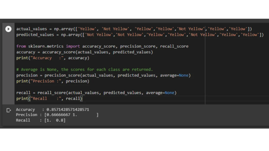
actual_values = np.array(['Yellow', 'Not Yellow', 'Yellow','Yellow','Not Yellow','Yellow','Yellow'])
predicted_values = np.array(['Not Yellow','Not Yellow','Yellow','Yellow','Not Yellow','Yellow','Yellow'])

from sklearn.metrics import accuracy_score, precision_score, recall_score
accuracy = accuracy_score(actual_values, predicted_values)
print("Accuracy   :", accuracy)

# Average is None, the scores for each class are returned.
precision = precision_score(actual_values, predicted_values, average=None)
print("Precision :", precision)

recall = recall_score(actual_values, predicted_values, average=None)
print("Recall    :", recall)
OUTPUT
Multi-Class Classification Confusion Matrix
A confusion matrix can be created for any number of classes (N X N). It is very similar to the binary classification we discussed earlier. The only difference is we need to calculate the values of TP, TF, FP, and FN in case of multi-class classification, direct representation is not achieved.
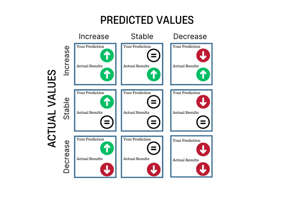
To understand Multi-class classification let us consider this example – You invested or are keeping an eye on a particular stock. There are three possibilities the price of the stock can go up (increase), can go down (decrease), or remain as it was the previous time you checked (stable). So the instinct you have are the predicted values and the results are the actual values. This can be represented using the confusion matrix.
Implementing Confusion Matrix for Multi-Class Classification
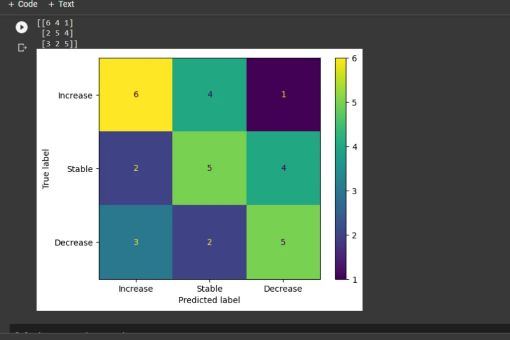
actual_value = [0]*11 + [1]*11 + [2]*10
predicted_value = [0]*6 + [1]*4 + [2]*1 + [0]*2 + [1]*5 + [2]*4 + [0]*3 + [1]*2 + [2]*5

confusion_mat = metrics.confusion_matrix(actual_value, predicted_value)
CM_view = metrics.ConfusionMatrixDisplay(confusion_matrix = confusion_mat, display_labels = ["Increase", "Stable", "Decrease"])

m = metrics.confusion_matrix(actual_value, predicted_value, labels=[0,1,2])
print(m)

CM_view.plot()
plot.show()
OUTPUT
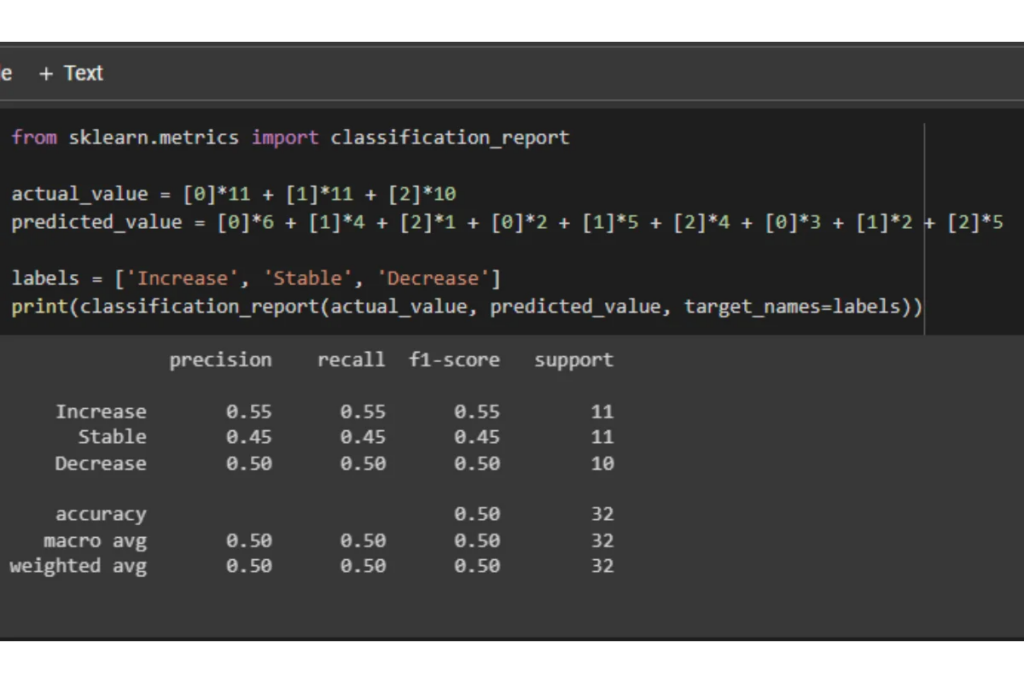
We can calculate the factors like accuracy, precision, etc for multi-class classification also. Another interesting thing we can do is build a text report showing the main classification metrics. To do so we import the classification_report() from the sklearn.metrics package.
from sklearn.metrics import classification_report

actual_value = [0]*11 + [1]*11 + [2]*10
predicted_value = [0]*6 + [1]*4 + [2]*1 + [0]*2 + [1]*5 + [2]*4 + [0]*3 + [1]*2 + [2]*5

labels = ['Increase', 'Stable', 'Decrease']
print(classification_report(actual_value, predicted_value, target_names=labels))
OUTPUT
Conclusion and Further Learning
In this article, we studied what is Confusion Matrix, how is it helpful, and how to implement it in the Python programming language. We looked at different examples to understand the implementation of the confusion matrix for both binary classifications as well as for multi-class classifications.
To learn from more such detailed and easy-to-understand articles on various topics related to deep learning and Python programming language, visit here.
References
Wikipedia – Confusion Matrix
Sklearn.metrics User Guide