
New to Rust? Grab our free Rust for Beginners eBook Get it free →
Gaussian Kernel Matrix in Python: Applications, Creation, and Visualization

While working with machine learning algorithms you may have come across the term Gaussian kernel, especially in the context of image processing, computer vision, and various other fields in machine learning. In simple terms, the Gaussian kernel is a square matrix used to represent the distances between various points, by prioritizing the points that are in closer proximity to the central point. In this article, we’ll try to understand what a Gaussian kernel really is, what it’s used for, and see how we can create one using NumPy. We’ll also look at how the Gaussian matrix we have generated can be visualized using Matplotlib.
What is a Gaussian Kernel and Why Do We Need It?
The Gaussian kernel is a function used to represent the distance between a set of neighboring points from a central point by assigning higher weights to the closer points and lesser weights to the distant points. This function relates closely to the Gaussian distribution in the sense that the points which ultimately make up the matrix are calculated on the basis of Gaussian distribution.
In short, the Gaussian kernel transforms the data points obtained by the Gaussian distribution into a higher dimensional space (like a 2D or 3D space). The matrix obtained resembles the bell-shaped curve obtained by the Gaussian distribution, assuming that the peak of the curve is the point assigned the highest weight. A bit tricky, but let us try visualizing it.
Imagine your Gaussian kernel to be a 3×3 grid. The centermost square would have the highest weightage which decreases as we go farther away from the center. Let’s look at an example.
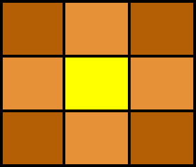
Here, the highest intensity is given to the yellow square in the center. The adjacent orange squares are less intense as compared to the highly intense yellow peak at the center. As the brown squares are furthest away from the center, they appear to be the least intense.
Now that we have understood what a Gaussian kernel is you are probably wondering what we can use it for. Let us look at some of its applications.
Applications of Gaussian Kernel
The Gaussian kernel can prove to be a powerful tool when it comes to data transformation and modelling in machine learning due to its ability to analyze complex patterns. It is also used in various machine learning algorithms to make predictions. Some of its common applications are as follows:
- Processing Images: Gaussian kernels are widely used for image processing tasks like image smoothening or blurring. They are typically used to reduce the noise present in the image and remove the grainy appearance, making the image smoother. This is done by replacing the intensity of each pixel with that of its adjacent ones, where the intensity is determined using the Gaussian kernel function.
- SVM (Support Vector Machines): SVM is a commonly used supervised machine learning algorithm that is mainly used for classification and regression tasks. Its main goal is to classify higher-dimensional spaces into different classes. The Gaussian kernel comes in handy to create these decision boundaries between these classes, which ultimately creates the hyperplane.
- Estimating Kernel Density: Gaussian kernels are used in the estimation of kernel density which is a method used to roughly estimate the probability density function of a random variable.
These are only some of the many applications the Gaussian kernel serves. It proves to be a versatile tool that aids in many fields ranging from computer vision to statistical analysis to name a few.
Mathematical Representation of Gaussian Kernel Matrix
The Gaussian kernel matrix is based on its Gaussian distribution curve. The formula to calculate the Gaussian kernel at an arbitrary point K(x,y) is as follows:

Or,
K(x, y) = (1 / (2 * pi * sigma^2)) * exp(-(x^2 + y^2) / (2 * sigma^2))
Here, sigma (σ) denotes the standard deviation of the distribution, which is used to determine how scattered or smooth the matrix should be, and |x-y| denotes the absolute distance between the points x and y.
The result obtained from the formula is a value that lies between 0 and 1, where the higher value signifies lesser distance (higher weightage) and the lower value signifies greater distance.
Now let’s see how we can use this formula to implement a Gaussian kernel matrix.
Implementing the Gaussian Kernel Using NumPy
In order to create a Gaussian kernel matrix we must calculate the value of the Gaussian kernel for every point in the given dataset. This can be achieved using various functions from Python’s NumPy library. NumPy is used to work with arrays and multidimensional matrices on which various operations can be performed.
Let us write a function gaussian_kernel() which will generate a Gaussian kernel matrix.
Code:
import numpy as np

def gaussian_kernel(kernel_size, sigma):
    kernel = np.fromfunction(lambda x, y: (1 / (2 * np.pi * sigma**2)) * np.exp(-((x - kernel_size//2)**2 + (y - kernel_size//2)**2) / (2 * sigma**2)), (kernel_size, kernel_size))
    normal = kernel / np.sum(kernel)
    return normal

kernel_size = 5
sigma = 1.0
gaussian_matrix = gaussian_kernel(kernel_size, sigma)
print(gaussian_matrix)
Here, we first import the NumPy as np using the import statement. Then we define the gaussian_kernel() function which takes in two arguments, kernel_size used to denote the dimensions of the kernel (3×3, 5×5, etc.), and sigma which denotes the smoothness of the matrix obtained.
Then we declare a variable kernel, which stores the Gaussian kernel value obtained using the formula. We use NumPy’s built-in function fromfunction() which returns a matrix based on the function that we have given as input. We input the Gaussian kernel formula into fromfunction().
In fromfunction() we use the lambda function which is essentially used to define an anonymous function. Here, we input a nameless function that computes the distance between each point (x,y) of the Gaussian distribution.
The syntax of a lambda function is as follows:
lambda arguments : expression
We then divide the kernel by the sum of all the elements (which is calculated using NumPy’s sum() function) of the kernel matrix in order to normalize it which ensures that the sum of the values in the matrix is 1. This value is stored in a variable normal, and returned by the gaussian_kernel() function.
Finally, we assign the kernel_size value and value of sigma, which are passed as arguments to the gaussian_kernel() function to generate the matrix.
Output:
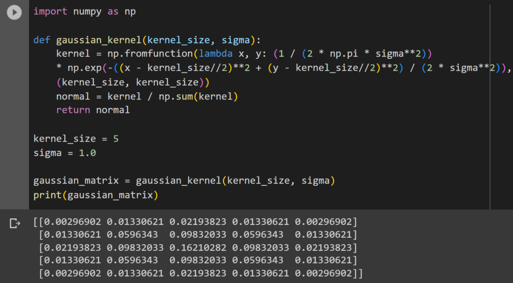
The centermost value is the greatest and the values decrease towards the ends. We can observe that the values at the corners of the matrix are the least.
Now that we have generated the Gaussian kernel we can also visualize it using the Matplotlib library.
Visualizing the Gaussian Kernel Using Matplotlib
Matplotlib is a Python library used for data visualization using charts and graphs. We can use this library to visualize our Gaussian kernel in the form of a grid.
Code:
import matplotlib.pyplot as plt

plt.imshow(gaussian_matrix, cmap='viridis')
plt.title('Gaussian Kernel Matrix')
plt.colorbar()
plt.show()
First, we import the matplotlib library as plt. We then use the imshow() in-built function from matplotlib which lets us visualize our Gaussian kernel matrix in the form of a grid made up of colored pixels. We pass 3 arguments into the imshow() function, the first one being the Gaussian matrix, the second cmap, which signifies the colormap that will be used to visualize the grid pixels. ‘viridis’ denotes the lowest values in blue and the highest values in yellow.
Finally, we can then give a title to our graph using title() and color bar using colorbar() which indicates what value each color of the graph denotes and then we can display the graph using the show() function.
Output:
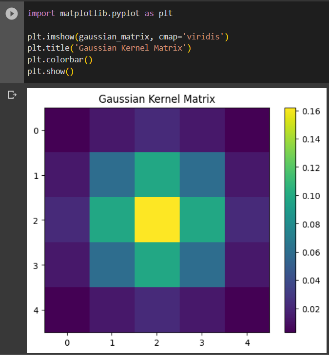
Here, we can see that the centermost point has the highest intensity, and as we go further away from the center the intensity decreases. Therefore, we can prove that the matrix generated is indeed a Gaussian kernel matrix.
Conclusion
In the world of machine learning, Gaussian matrices are a great tool that can help us perform many complex tasks that involve the analysis of patterns. Along with the help of the NumPy library we have seen that generating higher-dimensional matrices has been reduced to a comparatively easier task. We have also seen various applications of the Gaussian kernel matrix in the real world and how we can implement one ourselves quite easily. We have also explored the Matplotlib library which helps us visualize the matrix we have generated.
Reference