Neural Network Basics and a Python Build From Scratch

A neural network becomes easier to understand when you reduce it to the numbers it changes during training. My saved execution receipt records a complete run with Python 3.14.6 and NumPy 2.5.1, connecting neural network basics such as weights, activations, loss, and backpropagation to one result.

Neural network basics begin with one calculation

A neuron receives numeric inputs, multiplies them by learned weights, adds a bias, and sends the sum through an activation function. Written compactly, its input is z = xW + b and its output is a = f(z).

The weight controls how strongly an input affects the neuron. The bias shifts the point where the neuron responds, which lets the model fit data that does not pass through the origin.

Inputs, weights, and biases have distinct jobs

Inputs are the features you provide, such as pixel values or measurements. Weights and biases are parameters, meaning training changes them rather than asking you to choose every value by hand.

A layer evaluates several neurons together, and NumPy represents the inputs and weights as matrices so matrix multiplication computes many weighted sums in one operation.

An activation function adds nonlinearity

If every layer performs only multiplication and addition, several layers collapse into one linear transformation. A nonlinear activation prevents that collapse and lets the network describe curved decision boundaries.

The example below uses the sigmoid function, which maps any input to a value between 0 and 1. Sigmoid makes the final value easy to read as a binary-class probability, although rectified linear unit (ReLU) activations are more common in hidden layers of larger networks.

What a neural network learns during training

Training repeats a forward pass, a loss calculation, a backward pass, and a parameter update. Each stage answers a different question about the model.

Stage	What happens	Why it matters
Forward pass	Inputs travel through the layers to produce predictions.	You can measure the model’s present behavior.
Loss	A function compares predictions with target values.	One number expresses how wrong the batch is.
Backpropagation	The chain rule computes how each parameter affects the loss.	You get a gradient for every weight and bias.
Gradient descent	Parameters move opposite their gradients.	The next forward pass should have lower loss.

Backpropagation does not update the parameters by itself. It calculates gradients, while gradient descent uses those gradients and a learning rate to choose the size of each update.

A high learning rate can jump past a useful solution. A very low one can make progress needlessly slow, so this value is a training choice rather than a property the network discovers.

Build a neural network from scratch with NumPy

The exclusive OR (XOR) function is a compact test because it returns 1 when its two inputs differ and 0 when they match. A single linear decision boundary cannot separate its four cases, but a hidden layer can.

Create a fresh environment and install NumPy with these commands.

python -m venv .venv
source .venv/bin/activate
python -m pip install numpy

Save the following program as neural_network.py. It trains a network with two inputs, four hidden neurons, and one output neuron.

import numpy as np


def sigmoid(values):
    return 1.0 / (1.0 + np.exp(-values))


features = np.array([
    [0.0, 0.0],
    [0.0, 1.0],
    [1.0, 0.0],
    [1.0, 1.0],
])
targets = np.array([[0.0], [1.0], [1.0], [0.0]])

rng = np.random.default_rng(7)
weights_hidden = rng.normal(0.0, 0.5, size=(2, 4))
bias_hidden = np.zeros((1, 4))
weights_output = rng.normal(0.0, 0.5, size=(4, 1))
bias_output = np.zeros((1, 1))

learning_rate = 1.0
sample_count = features.shape[0]

for epoch in range(10_001):
    hidden_input = features @ weights_hidden + bias_hidden
    hidden_output = sigmoid(hidden_input)
    output_input = hidden_output @ weights_output + bias_output
    predictions = sigmoid(output_input)

    epsilon = 1e-12
    loss = -np.mean(
        targets * np.log(predictions + epsilon)
        + (1.0 - targets) * np.log(1.0 - predictions + epsilon)
    )

    output_error = (predictions - targets) / sample_count
    gradient_weights_output = hidden_output.T @ output_error
    gradient_bias_output = np.sum(output_error, axis=0, keepdims=True)

    hidden_error = (output_error @ weights_output.T) * hidden_output * (1.0 - hidden_output)
    gradient_weights_hidden = features.T @ hidden_error
    gradient_bias_hidden = np.sum(hidden_error, axis=0, keepdims=True)

    weights_output -= learning_rate * gradient_weights_output
    bias_output -= learning_rate * gradient_bias_output
    weights_hidden -= learning_rate * gradient_weights_hidden
    bias_hidden -= learning_rate * gradient_bias_hidden

    if epoch % 2_000 == 0:
        print(f"epoch={epoch:5d} loss={loss:.6f}")

hidden_output = sigmoid(features @ weights_hidden + bias_hidden)
predictions = sigmoid(hidden_output @ weights_output + bias_output)
classes = (predictions >= 0.5).astype(int)

print("\nXOR predictions")
for inputs, probability, label in zip(features.astype(int), predictions, classes):
    print(f"input={inputs.tolist()} probability={probability.item():.4f} class={label.item()}")

Run the program with the active environment.

python neural_network.py

The loss falls from about 0.694 to 0.001, and the thresholded predictions match all four XOR targets. My execution receipt captures the command run from the saved source and its unedited output.

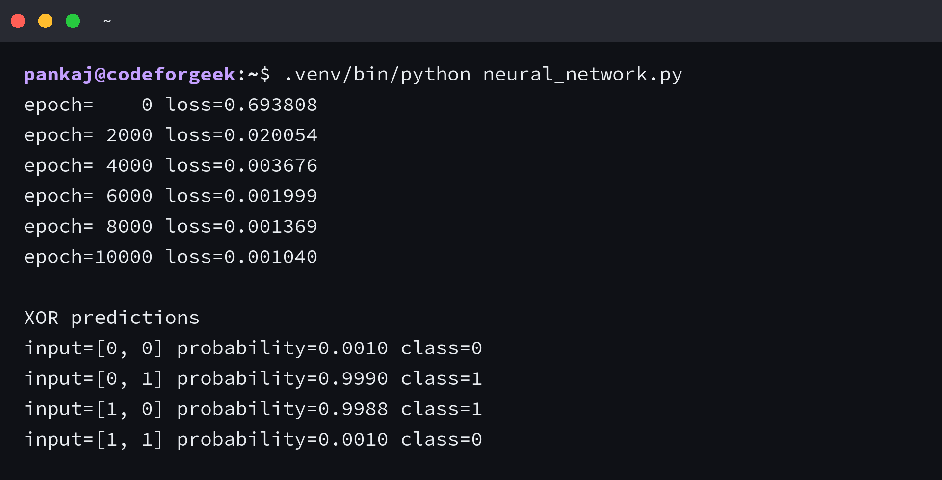
epoch=    0 loss=0.693808
epoch= 2000 loss=0.020054
epoch= 4000 loss=0.003676
epoch= 6000 loss=0.001999
epoch= 8000 loss=0.001369
epoch=10000 loss=0.001040

XOR predictions
input=[0, 0] probability=0.0010 class=0
input=[0, 1] probability=0.9990 class=1
input=[1, 0] probability=0.9988 class=1
input=[1, 1] probability=0.0010 class=0

Read the array shapes before reading the formulas

Most shape errors become obvious when you track how many samples and neurons each array represents. The four XOR rows form the sample dimension.

Array	Shape	Meaning
features	(4, 2)	Four samples with two inputs each
weights_hidden	(2, 4)	Every input connects to four hidden neurons
bias_hidden	(1, 4)	One bias for each hidden neuron
weights_output	(4, 1)	Four hidden outputs connect to one result
predictions	(4, 1)	One probability for each sample

The forward pass transforms features into predictions

The first matrix multiplication combines two input values into four hidden weighted sums. Sigmoid transforms those sums, and the second matrix multiplication combines the hidden outputs into one value per sample.

The seeded random number generator makes the initialization repeatable. Starting every weight at zero would make hidden neurons receive identical gradients, so they would continue learning the same function instead of dividing the work.

Binary cross-entropy measures the prediction error

Binary cross-entropy assigns a large penalty when the network gives high confidence to the wrong class. The epsilon value keeps logarithms away from zero, where the calculation is undefined.

Mean squared error can train simple networks too, but binary cross-entropy matches this binary classification task more directly, so the loss choice should follow the output and the task rather than habit.

The backward pass follows dependencies in reverse

For sigmoid output with binary cross-entropy, the derivative at the output simplifies to predictions minus targets. Dividing by the sample count keeps the gradient scale consistent with the mean loss.

The output gradient flows through weights_output to reach the hidden layer, while multiplying by hidden_output times one minus hidden_output applies the sigmoid derivative and transposed matrix multiplications produce gradients with the same shapes as the weights.

Gradient descent changes every parameter

Each update subtracts the learning rate multiplied by a gradient because a positive gradient means increasing that parameter would increase loss locally, so subtraction moves it in the reducing direction.

The loop prints loss at intervals, which gives you a quick training check, but a falling training loss confirms optimization only on this tiny dataset and does not prove that a model will generalize to unseen data.

Failure boundaries worth checking

This XOR network is an explanation tool, not a production architecture. Its entire dataset is used for training and evaluation, so the final accuracy says nothing about performance on new samples.

• Loss stays near 0.693. Check that gradients reach both layers and that parameters change after each iteration.
• Loss becomes not a number. Reduce the learning rate and keep logarithm inputs away from zero.
• Every prediction is similar. Confirm that hidden weights did not all start with the same value.
• Training improves but validation worsens. The network may be fitting noise or memorizing the training set.
• Gradients become tiny in a deep sigmoid network. Saturated sigmoid units pass little gradient backward, which is one reason larger hidden stacks often use ReLU-family activations.

Gradient checking can catch derivative mistakes by perturbing one parameter by a small positive and negative amount, estimating the loss slope from those two runs, and comparing it with the backpropagated gradient before trusting a custom training loop.

Move from the small network to practical projects

Writing one network with NumPy shows where each number comes from. For larger models, an automatic differentiation framework records operations and computes the same backward dependencies for you.

You can compare that next layer of tooling in the machine learning frameworks for web development overview. Frameworks remove much of the derivative bookkeeping, but you still need the forward-pass, loss, and gradient model to diagnose poor training.

If you want to check the terminology before moving on, the machine learning question set covers core concepts in a different format. Use it after you can explain why XOR needs a hidden nonlinear layer, not as a substitute for running the network.

Keep one training rule

A neural network learns parameters that reduce a chosen loss. When a model behaves badly, inspect that chain in order: inputs, weighted sums, activations, predictions, loss, gradients, and updates.

Change one element of the XOR program next, such as the hidden width or learning rate, then compare the loss trace. That controlled edit gives you a stronger mental model than adding more layers before you can explain the first two.